Notes on Optimizing Non-Differentiable (but Convex) Functions: Subgradients, and Projected and Proximal Methods

$$ \newcommand{\bzero}{\mathbf{0}} \newcommand{\ba}{\mathbf{a}}\newcommand{\bA}{\mathbf{A}} \newcommand{\bb}{\mathbf{b}}\newcommand{\bB}{\mathbf{B}} \newcommand{\bc}{\mathbf{c}}\newcommand{\bC}{\mathbf{C}} \newcommand{\bd}{\mathbf{d}}\newcommand{\bD}{\mathbf{D}} \newcommand{\be}{\mathbf{e}}\newcommand{\bE}{\mathbf{E}} \newcommand{\bff}{\mathbf{f}}\newcommand{\bF}{\mathbf{F}} \newcommand{\bg}{\mathbf{g}}\newcommand{\bG}{\mathbf{G}} \newcommand{\bh}{\mathbf{h}}\newcommand{\bH}{\mathbf{H}} \newcommand{\bi}{\mathbf{i}}\newcommand{\bI}{\mathbf{I}} \newcommand{\bj}{\mathbf{j}}\newcommand{\bJ}{\mathbf{J}} \newcommand{\bk}{\mathbf{k}}\newcommand{\bK}{\mathbf{K}} \newcommand{\bl}{\mathbf{l}}\newcommand{\bL}{\mathbf{L}} \newcommand{\bm}{\mathbf{m}}\newcommand{\bM}{\mathbf{M}} \newcommand{\bn}{\mathbf{n}}\newcommand{\bN}{\mathbf{N}} \newcommand{\bo}{\mathbf{o}}\newcommand{\bO}{\mathbf{O}} \newcommand{\bp}{\mathbf{p}}\newcommand{\bP}{\mathbf{P}} \newcommand{\bq}{\mathbf{q}}\newcommand{\bQ}{\mathbf{Q}} \newcommand{\br}{\mathbf{r}}\newcommand{\bR}{\mathbf{R}} \newcommand{\bs}{\mathbf{s}}\newcommand{\bS}{\mathbf{S}} \newcommand{\bt}{\mathbf{t}}\newcommand{\bT}{\mathbf{T}} \newcommand{\bu}{\mathbf{u}}\newcommand{\bU}{\mathbf{U}} \newcommand{\bv}{\mathbf{v}}\newcommand{\bV}{\mathbf{V}} \newcommand{\bw}{\mathbf{w}}\newcommand{\bW}{\mathbf{W}} \newcommand{\indep}{\perp \!\!\! \perp} \newcommand{\bx}{\mathbf{x}}\newcommand{\bX}{\mathbf{X}} \newcommand{\by}{\mathbf{y}}\newcommand{\bY}{\mathbf{Y}} \newcommand{\bz}{\mathbf{z}}\newcommand{\bZ}{\mathbf{Z}} \newcommand{\balpha}{\boldsymbol{\alpha}}\newcommand{\bAlpha}{\boldsymbol{\Alpha}} \newcommand{\bbeta}{\boldsymbol{\beta}}\newcommand{\bBeta}{\boldsymbol{\Beta}} \newcommand{\bgamma}{\boldsymbol{\gamma}}\newcommand{\bGamma}{\boldsymbol{\Gamma}} \newcommand{\bdelta}{\boldsymbol{\delta}}\newcommand{\bDelta}{\boldsymbol{\Delta}} \newcommand{\bepsilon}{\boldsymbol{\epsilon}}\newcommand{\bEpsilon}{\boldsymbol{\Epsilon}} \newcommand{\bzeta}{\boldsymbol{\zeta}}\newcommand{\bZeta}{\boldsymbol{\Zeta}} \newcommand{\beeta}{\boldsymbol{\eta}}\newcommand{\bEta}{\boldsymbol{\Eta}} % \beta already taken \newcommand{\btheta}{\boldsymbol{\theta}}\newcommand{\bTheta}{\boldsymbol{\Theta}} \newcommand{\biota}{\boldsymbol{\iota}}\newcommand{\bIota}{\boldsymbol{\Iota}} \newcommand{\bkappa}{\boldsymbol{\kappa}}\newcommand{\bKappa}{\boldsymbol{\Kappa}} \newcommand{\blambda}{\boldsymbol{\lambda}}\newcommand{\bLambda}{\boldsymbol{\Lambda}} \newcommand{\bmu}{\boldsymbol{\mu}}\newcommand{\bMu}{\boldsymbol{\Mu}} \newcommand{\bnu}{\boldsymbol{\nu}}\newcommand{\bNu}{\boldsymbol{\Nu}} \newcommand{\bxi}{\boldsymbol{\xi}}\newcommand{\bXi}{\boldsymbol{\Xi}} \newcommand{\bomikron}{\boldsymbol{\omikron}}\newcommand{\bOmikron}{\boldsymbol{\Omikron}} \newcommand{\bpi}{\boldsymbol{\pi}}\newcommand{\bPi}{\boldsymbol{\Pi}} \newcommand{\brho}{\boldsymbol{\rho}}\newcommand{\bRho}{\boldsymbol{\Rho}} \newcommand{\bsigma}{\boldsymbol{\sigma}}\newcommand{\bSigma}{\boldsymbol{\Sigma}} \newcommand{\btau}{\boldsymbol{\tau}}\newcommand{\bTau}{\boldsymbol{\Tau}} \newcommand{\bypsilon}{\boldsymbol{\ypsilon}}\newcommand{\bYpsilon}{\boldsymbol{\Ypsilon}} \newcommand{\bphi}{\boldsymbol{\phi}}\newcommand{\bPhi}{\boldsymbol{\Phi}} \newcommand{\bchi}{\boldsymbol{\chi}}\newcommand{\bChi}{\boldsymbol{\Chi}} \newcommand{\bpsi}{\boldsymbol{\psi}}\newcommand{\bPsi}{\boldsymbol{\Psi}} \newcommand{\bomega}{\boldsymbol{\omega}}\newcommand{\bOmega}{\boldsymbol{\Omega}} \newcommand{\nA}{\mathbb{A}} \newcommand{\nB}{\mathbb{B}} \newcommand{\nC}{\mathbb{C}} \newcommand{\nD}{\mathbb{D}} \newcommand{\nE}{\mathbb{E}} \newcommand{\nF}{\mathbb{F}} \newcommand{\nG}{\mathbb{G}} \newcommand{\nH}{\mathbb{H}} \newcommand{\nI}{\mathbb{I}} \newcommand{\nJ}{\mathbb{J}} \newcommand{\nK}{\mathbb{K}} \newcommand{\nL}{\mathbb{L}} \newcommand{\nM}{\mathbb{M}} \newcommand{\nN}{\mathbb{N}} \newcommand{\nO}{\mathbb{O}} \newcommand{\nP}{\mathbb{P}} \newcommand{\nQ}{\mathbb{Q}} \newcommand{\nR}{\mathbb{R}} \newcommand{\nS}{\mathbb{S}} \newcommand{\nT}{\mathbb{T}} \newcommand{\nU}{\mathbb{U}} \newcommand{\nV}{\mathbb{V}} \newcommand{\nW}{\mathbb{W}} \newcommand{\nX}{\mathbb{X}} \newcommand{\nY}{\mathbb{Y}} \newcommand{\nZ}{\mathbb{Z}} \newcommand{\cA}{\mathcal{A}} \newcommand{\cB}{\mathcal{B}} \newcommand{\cC}{\mathcal{C}} \newcommand{\cD}{\mathcal{D}} \newcommand{\cE}{\mathcal{E}} \newcommand{\cF}{\mathcal{F}} \newcommand{\cG}{\mathcal{G}} \newcommand{\cH}{\mathcal{H}} \newcommand{\cI}{\mathcal{I}} \newcommand{\cJ}{\mathcal{J}} \newcommand{\cK}{\mathcal{K}} \newcommand{\cL}{\mathcal{L}} \newcommand{\cM}{\mathcal{M}} \newcommand{\cN}{\mathcal{N}} \newcommand{\cO}{\mathcal{O}} \newcommand{\cP}{\mathcal{P}} \newcommand{\cQ}{\mathcal{Q}} \newcommand{\cR}{\mathcal{R}} \newcommand{\cS}{\mathcal{S}} \newcommand{\cT}{\mathcal{T}} \newcommand{\cU}{\mathcal{U}} \newcommand{\cV}{\mathcal{V}} \newcommand{\cW}{\mathcal{W}} \newcommand{\cX}{\mathcal{X}} \newcommand{\cY}{\mathcal{Y}} \newcommand{\cZ}{\mathcal{Z}} \DeclareMathOperator*{\argmax}{argmax~} \DeclareMathOperator*{\argmin}{argmin~} \DeclareMathOperator*{\Tr}{Tr} \DeclareMathOperator*{\Bias}{Bias} \DeclareMathOperator*{\Var}{Var} \newcommand{\Perp}{\perp\!\!\! \perp} \let\dsad\d \renewcommand\d{\, \mathrm{d}} \newcommand{\R}{\mathbb{R}} \newcommand{\N}{\mathbb{N}} \newcommand{\E}{\mathbb{E}} \newcommand{\Eb}[1]{\mathbb{E} \left[ #1 \right]} \newcommand{\F}{\mathcal{F}} \newcommand{\X}{\mathcal{X}} \newcommand{\vocab}[1]{\textbf{\color{blue} #1}} \newcommand{\norm}[1]{\left\lVert#1\right\rVert} \newcommand{\inner}[2]{ \left \langle #1, #2 \right \rangle } \newcommand{\ibra}[1]{\llbracket #1 \rrbracket} \newenvironment{nalign}{ \begin{equation} \begin{aligned} }{ \end{aligned} \end{equation} \ignorespacesafterend } \newcommand{\icol}[1]{ \left(\begin{smallmatrix}#1\end{smallmatrix}\right)% } \newcommand{\cc}[1]{\overline{#1}} \newcommand{\tr}[1]{\text{tr} \left( #1 \right)} \newcommand{\aff}{\text{aff} \,} \newcommand{\ri}{\text{ri} \, } \newcommand{\rb}{\text{rb} \, } \newcommand{\cl}{\text{cl} \, } \newcommand{\conv}{\text{conv} \, } \newcommand{\irow}[1]{ \begin{smallmatrix}(#1)\end{smallmatrix}% } \newcommand\abs[1]{\left \lvert #1 \right \rvert} $$

In this post I go over an important topic: Non-Smooth Convex Optimization. In this case we will be dealing with convex, but not smooth functions. In particular, here we do not assume that the function is differentiable everywhere, but is continuous.

Here I focus mostly on the practical aspect of the topic, and leave the inspection of the mathematical intricacies for a different post. I base most of the material from (missing reference), (missing reference), and from a local course at the University of Tübingen given by Peter Ochs (missing reference).

Subdifferential

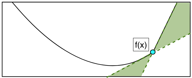
A key player in our setting will be the subdifferential – a analog of the gradient for non-differentiable continuous convex functions. It is a function that for any point in the input space, produces a set of vectors such that the subgradient inequality, defined below, holds.

Definition (Subgradient Inequality) For a convex function $f : \R^n \to \R$, we say that $\bv$ is a subgradient of $f$ at $\bx$ if it holds that

\[\begin{equation} \begin{split} f(\by) \geq f(\bx) + \inner{\bv}{\by - \bx} \quad \forall \by. \end{split} \end{equation}\]

To see how this is related to the differentiable $f$ case, remember that then for any $\bx, \by$ it holds that $f(\by) \geq f(\bx) + \inner{\nabla f(\bx)}{\by - \bx}$. In that case, the it holds that the gradient satisfies the subgradient inequality.

We can package the subgradients at individual points into a subdifferential, a function that maps points in the input space to the points that satisfy the subgradient inequality at that point.

Definition (Subdifferential) A subdifferential, denoted as $\partial f : \R^n \rightrightarrows \R$, is a set mapping, that maps points to the set of values that satisfy the subgradient inequality.

If the function is differentiable, we know that the gradient is a subset of the subdifferential. But what about the other way round? That is, are there any points that are not the gradient evaluated at some point that also satisfy the subgradient inequality? No, there are not.

Figure 1. Illustration of the linearizations at the point $x$ with the slopes that are given by the subdifferential at $x$. Source: (missing reference).

Key condition for subdifferential optimization

We will make use of the following little theorem, that similarly as in gradient optimization, states that a point $\bx$ is a global minimum iff $\bzero \in \partial f(\bx)$.

Theorem (Fermat’s Rule) A point $\bx$ is a global minimum of a convex function if $\bzero \in \partial f(\bx)$.

Proof. “$\Rightarrow$”: if $\bx$ is global minimum, then $\forall \by: f(\by) \geq f(\bx) = f(\bx) + \inner{\bzero}{\by - \bx}$. “ $\Leftarrow$”: if $\bzero \in \partial f(\bx)$, then $f(\by) \geq f(\bx) + \inner{\bzero}{\by - \bx} = f(\bx)$.

Application of subdifferential optimization: regularization and sparsity

A nice application of the subdifferential optimization is showing that L1 regularization has a non-zero-width interval. In contrast, if L2 weight regularization is used, this leads to an unique condition for a weight to be exactly zero. We illustrate both of those cases.

Example (L2 regualarization does not lead to a sparse solution). Consider a regression problem given data $X \in \R^{n \times m}$ ($n$ datapoints, $m$ features), the targets $Y \in \R^{n \times 1}$, and a set of features/weights we are optimizing $\bw \in \R^{m \times 1}$, expressed as an optimization problem with the L2 regularized loss

\[\begin{equation} \begin{split} \cL(\bw) &= \norm{X\bw - Y}_2^2 + \lambda \norm{\bw}_2^2 \\ &= \sum_{i}^n (\bx_i^\intercal \bw - y_i)^2 + \lambda \sum_i^m w_i^2 . \end{split} \end{equation}\]

The loss is a convex function. If the optimal weight $w_j$ is exactly 0, then it must hold that $ \left( \frac{\partial}{\partial w_j} \cL(\bw) \right ) \Big \lvert_{w_j = 0} = 0$. Noting that

\[\begin{equation} \begin{split} & \left(\frac{\partial}{\partial w_j} \cL(\bw) \right)\Bigg|_{w_j = 0} = 0 \\ \Rightarrow \quad & \sum_i (\bx_i^\intercal \bw - y_i) x_{ij} = 0 \\ \Rightarrow \quad & \sum_i \bx_i^\intercal \bw x_{ij} - \sum_i y_i x_{ij} = 0 \\ \Rightarrow \quad & \bw^\intercal \sum_i \bx_i x_{ij} - \sum_i y_i x_{ij} = 0 \\ \Rightarrow \quad & \bw^\intercal X^\intercal \bx_{*j} - \by^\intercal \bx_{*j} = 0 \\ \Rightarrow \quad & (\bw^\intercal X^\intercal - \by^\intercal) \bx_{*j} = 0, \end{split} \end{equation}\]

where $\bx_{*j}$ denotes the $j$-th column of the matrix $X$. We can see that for $w_i = 0$ to be optimal, the signed error of our prediction must be exactly orthogonal to the $j$-th column of the input matrix $X$. This can happen, for example, if the $j$-th feature is completely irrelevant, in the sense that 0 erorr can be reached using all the other features. But if the feature vector for all the points is not orthogonal to the signed error, the optimal weight $w_j$ will not be zero.

In contrast, the behavior of optimizing the loss in case L1 regularization is used can be understood by writing down the criterion to satisfy Fermat’s rule. Since this will involve subdifferential of L1 norm (absolute value for the case here), we can find it by writing down the subgradient inequality for the case $x = 0$:

\[\begin{equation} \begin{split} & f(y) \geq f(x) + a(y - x) \\ \Rightarrow \quad & \abs{y} \geq a y \\ \Rightarrow \quad & \frac{\abs{y}}{y} \geq a \\ \Rightarrow \quad & a \in [-1, 1]. \\ \end{split} \end{equation}\]

With this in mind, we find the condition for a weight in the regression problem to be 0 in the following example.

Example (L1 regularizaiton leads to a potentially sparse solution). Here we consider the same problem setting as in the previous example, only imposing L1 regularization on the weights as

\[\begin{equation} \begin{split} \cL(\bw) &= \norm{X\bw - Y}_2^2 + \lambda \norm{\bw}_1^2 \\ &= \sum_{i}^n (\bx_i^\intercal \bw - y_i)^2 + \lambda \sum_i^m |w_i| . \end{split} \end{equation}\]

Once again, we can find the condition for which the optimal weight is zero, i.e. $w_j = 0$, by using the Fermat’s rule by finding points for which 0 is in the subdifferential. With slight abuse of notation, and by defining a one-dim function with a fixed $\bw$, $\cL_j(w_j)$ , we find the optimal

\[\begin{equation} \begin{split} & 0 \in \partial \cL_j (w_j) |_{w_j = 0} \\ \Rightarrow \quad & 0 \in \left ( \bw^\intercal X^\intercal - \by^\intercal) \bx_{*j} + \lambda [-1, 1] \right )\Big |_{w_j = 0} \\ \Rightarrow \quad & \lambda [-1, 1] \in (\bw^\intercal X^\intercal - \by^\intercal) \bx_{*j} \\ \Rightarrow \quad & \abs{(\bw^\intercal X^\intercal - \by^\intercal) \bx_{*j}} \leq \lambda. \\ \end{split} \end{equation}\]

This exactly shows that there is an interval of solutions where the optimal weight is exactly zero.

Optimization through Subgradient Method

One way to extend Gradient Method to non-smooth problem discussed here is to replace all instances of gradients with vectors from the subgradient. This can be formalized as follows.

Method (Subgradient Method) For a convex function $f: \R^n \to \R$, a step size $\tau > 0$, and a starting point $\bx^0$, Subgradient Method at each iteration step $t$ updates the current iterate from the previous step $\bx_{t-1}$ by the update rule $\bx^t := \bx^{t-1} - \tau \bv$, where $\bv$ is any subgradient of $\bx^{t-1}$, i.e. $\bv \in \partial f(\bx^{t-1})$.

Convergence of Subgradient Method

Turns out that using constant learning step $\tau$, we can get within $\cO(\alpha)$ margin of error. However, the method does not converge unless we use variable step size (e.g. by decaying it).

In order to show the convergence, we need to adjust our assumptions about the functions we optimize. In the differentiable $f$ case, we assumed gradients to be L-smooth. Since in this case differentiablity is not a given, we instead require that $f$ is Lipshitz-continuous. This will then turn out to show that the gradient is bounded by the same Lipshitz constant.

Definition (Lipshitz Contuinuity) A function $f$ is Lipshitz-continuous if there exists $L > 0$ s.t. $\forall \bx, \by \in \text{dom } f$, it holds that

\[\begin{equation} \begin{split} \abs{f(\by) - f(\bx)} \leq L \norm{\by - \bx}. \end{split} \end{equation}\]

Assuming a Lipshitz-continuous convex function $f$, we can then show the boundedness of the subdifferential for all points in the domain.

Figure 2. Intuition of L-continuity: the cone generated by linearization of slopes $-L$ and $L$ intersects the function at only a single point. (By Taschee - Own work, CC0)

Propostion (Function is Lipshitz if subradients bounded) A convex function is Lipshitz iff all subgradients are bounded $\sup_{\bv \in \text{im }\partial f } \norm{\bv} \leq m$

Proof. “$\Leftarrow$”: If $f$ is Lipshitz, then take $\by = \bx + \bv$, $\bv \in \partial f(\bx)$, and use the subgradient inequaliy to get

\[\begin{equation} \begin{split} & f(\by) \geq f(\bx) + \inner{\bv}{\by - \bx} \\ \Rightarrow \quad & f(\by) - f(\bx) \geq \norm{\bv}^2, \end{split} \end{equation}\]

but the right side can be bounded using Lipshitz continuity, and thus $\norm{\bv}^2 \leq m$.

”$\Rightarrow$”: if subgradients are bounded, rewrite the subgradient inequality and bound the inner product using Cauchy-Schwarz.

With this in mind, the convergence rate can be shown ( TODO: check this properly) to be slower than gradient descent on smooth functions (show here, for instance), but the arguments are similar to those made in differentiable case using Gradient Descent.

Conclusion

Subgradient method is applicable and guarantees convergence when the optimized function of interest is convex and the step size decays. However, the convergence rate is slower than for differentiable convex functions: $\cO(1/\sqrt{k})$ in subgradient method vs $\cO(1/k)$ is gradient descent.

However, if the optimization problem