$$ \newcommand{\bzero}{\mathbf{0}} \newcommand{\ba}{\mathbf{a}}\newcommand{\bA}{\mathbf{A}} \newcommand{\bb}{\mathbf{b}}\newcommand{\bB}{\mathbf{B}} \newcommand{\bc}{\mathbf{c}}\newcommand{\bC}{\mathbf{C}} \newcommand{\bd}{\mathbf{d}}\newcommand{\bD}{\mathbf{D}} \newcommand{\be}{\mathbf{e}}\newcommand{\bE}{\mathbf{E}} \newcommand{\bff}{\mathbf{f}}\newcommand{\bF}{\mathbf{F}} \newcommand{\bg}{\mathbf{g}}\newcommand{\bG}{\mathbf{G}} \newcommand{\bh}{\mathbf{h}}\newcommand{\bH}{\mathbf{H}} \newcommand{\bi}{\mathbf{i}}\newcommand{\bI}{\mathbf{I}} \newcommand{\bj}{\mathbf{j}}\newcommand{\bJ}{\mathbf{J}} \newcommand{\ind}{\perp\!\!\!\!\perp} \newcommand{\bk}{\mathbf{k}}\newcommand{\bK}{\mathbf{K}} \newcommand{\bl}{\mathbf{l}}\newcommand{\bL}{\mathbf{L}} \newcommand{\bm}{\mathbf{m}}\newcommand{\bM}{\mathbf{M}} \newcommand{\bn}{\mathbf{n}}\newcommand{\bN}{\mathbf{N}} \newcommand{\bo}{\mathbf{o}}\newcommand{\bO}{\mathbf{O}} \newcommand{\bp}{\mathbf{p}}\newcommand{\bP}{\mathbf{P}} \newcommand{\bq}{\mathbf{q}}\newcommand{\bQ}{\mathbf{Q}} \newcommand{\br}{\mathbf{r}}\newcommand{\bR}{\mathbf{R}} \newcommand{\bs}{\mathbf{s}}\newcommand{\bS}{\mathbf{S}} \newcommand{\bt}{\mathbf{t}}\newcommand{\bT}{\mathbf{T}} \newcommand{\bu}{\mathbf{u}}\newcommand{\bU}{\mathbf{U}} \newcommand{\bv}{\mathbf{v}}\newcommand{\bV}{\mathbf{V}} \newcommand{\bw}{\mathbf{w}}\newcommand{\bW}{\mathbf{W}} \newcommand{\bx}{\mathbf{x}}\newcommand{\bX}{\mathbf{X}} \newcommand{\Perp}{\perp\!\!\! \perp} \newcommand{\by}{\mathbf{y}}\newcommand{\bY}{\mathbf{Y}} \newcommand{\bz}{\mathbf{z}}\newcommand{\bZ}{\mathbf{Z}} \newcommand{\balpha}{\boldsymbol{\alpha}}\newcommand{\bAlpha}{\boldsymbol{\Alpha}} \newcommand{\bbeta}{\boldsymbol{\beta}}\newcommand{\bBeta}{\boldsymbol{\Beta}} \newcommand{\bgamma}{\boldsymbol{\gamma}}\newcommand{\bGamma}{\boldsymbol{\Gamma}} \newcommand{\bdelta}{\boldsymbol{\delta}}\newcommand{\bDelta}{\boldsymbol{\Delta}} \newcommand{\bepsilon}{\boldsymbol{\epsilon}}\newcommand{\bEpsilon}{\boldsymbol{\Epsilon}} \newcommand{\bzeta}{\boldsymbol{\zeta}}\newcommand{\bZeta}{\boldsymbol{\Zeta}} \newcommand{\beeta}{\boldsymbol{\eta}}\newcommand{\bEta}{\boldsymbol{\Eta}} % \beta already taken \newcommand{\btheta}{\boldsymbol{\theta}}\newcommand{\bTheta}{\boldsymbol{\Theta}} \newcommand{\biota}{\boldsymbol{\iota}}\newcommand{\bIota}{\boldsymbol{\Iota}} \newcommand{\bkappa}{\boldsymbol{\kappa}}\newcommand{\bKappa}{\boldsymbol{\Kappa}} \newcommand{\blambda}{\boldsymbol{\lambda}}\newcommand{\bLambda}{\boldsymbol{\Lambda}} \newcommand{\bmu}{\boldsymbol{\mu}}\newcommand{\bMu}{\boldsymbol{\Mu}} \newcommand{\bnu}{\boldsymbol{\nu}}\newcommand{\bNu}{\boldsymbol{\Nu}} \newcommand{\bxi}{\boldsymbol{\xi}}\newcommand{\bXi}{\boldsymbol{\Xi}} \newcommand{\bomikron}{\boldsymbol{\omikron}}\newcommand{\bOmikron}{\boldsymbol{\Omikron}} \newcommand{\bpi}{\boldsymbol{\pi}}\newcommand{\bPi}{\boldsymbol{\Pi}} \newcommand{\brho}{\boldsymbol{\rho}}\newcommand{\bRho}{\boldsymbol{\Rho}} \newcommand{\bsigma}{\boldsymbol{\sigma}}\newcommand{\bSigma}{\boldsymbol{\Sigma}} \newcommand{\btau}{\boldsymbol{\tau}}\newcommand{\bTau}{\boldsymbol{\Tau}} \newcommand{\bypsilon}{\boldsymbol{\ypsilon}}\newcommand{\bYpsilon}{\boldsymbol{\Ypsilon}} \newcommand{\bphi}{\boldsymbol{\phi}}\newcommand{\bPhi}{\boldsymbol{\Phi}} \newcommand{\bchi}{\boldsymbol{\chi}}\newcommand{\bChi}{\boldsymbol{\Chi}} \newcommand{\bpsi}{\boldsymbol{\psi}}\newcommand{\bPsi}{\boldsymbol{\Psi}} \newcommand{\bomega}{\boldsymbol{\omega}}\newcommand{\bOmega}{\boldsymbol{\Omega}} \newcommand{\nA}{\mathbb{A}} \newcommand{\nB}{\mathbb{B}} \newcommand{\nC}{\mathbb{C}} \newcommand{\nD}{\mathbb{D}} \newcommand{\nE}{\mathbb{E}} \newcommand{\nF}{\mathbb{F}} \newcommand{\nG}{\mathbb{G}} \newcommand{\nH}{\mathbb{H}} \newcommand{\nI}{\mathbb{I}} \newcommand{\nJ}{\mathbb{J}} \newcommand{\nK}{\mathbb{K}} \newcommand{\nL}{\mathbb{L}} \newcommand{\nM}{\mathbb{M}} \newcommand{\nN}{\mathbb{N}} \newcommand{\nO}{\mathbb{O}} \newcommand{\nP}{\mathbb{P}} \newcommand{\nQ}{\mathbb{Q}} \newcommand{\nR}{\mathbb{R}} \newcommand{\nS}{\mathbb{S}} \newcommand{\nT}{\mathbb{T}} \newcommand{\nU}{\mathbb{U}} \newcommand{\nV}{\mathbb{V}} \newcommand{\nW}{\mathbb{W}} \newcommand{\nX}{\mathbb{X}} \newcommand{\nY}{\mathbb{Y}} \newcommand{\nZ}{\mathbb{Z}} \newcommand{\cA}{\mathcal{A}} \newcommand{\cB}{\mathcal{B}} \newcommand{\cC}{\mathcal{C}} \newcommand{\cD}{\mathcal{D}} \newcommand{\cE}{\mathcal{E}} \newcommand{\cF}{\mathcal{F}} \newcommand{\cG}{\mathcal{G}} \newcommand{\cH}{\mathcal{H}} \newcommand{\cI}{\mathcal{I}} \newcommand{\cJ}{\mathcal{J}} \newcommand{\cK}{\mathcal{K}} \newcommand{\cL}{\mathcal{L}} \newcommand{\cM}{\mathcal{M}} \newcommand{\cN}{\mathcal{N}} \newcommand{\cO}{\mathcal{O}} \newcommand{\cP}{\mathcal{P}} \newcommand{\cQ}{\mathcal{Q}} \newcommand{\cR}{\mathcal{R}} \newcommand{\cS}{\mathcal{S}} \newcommand{\cT}{\mathcal{T}} \newcommand{\cU}{\mathcal{U}} \newcommand{\cV}{\mathcal{V}} \newcommand{\cW}{\mathcal{W}} \newcommand{\cX}{\mathcal{X}} \newcommand{\cY}{\mathcal{Y}} \newcommand{\cZ}{\mathcal{Z}} \DeclareMathOperator*{\argmax}{argmax~} \DeclareMathOperator*{\argmin}{argmin~} \DeclareMathOperator*{\Tr}{Tr} \DeclareMathOperator*{\Bias}{Bias} \DeclareMathOperator*{\Var}{Var} \newcommand{\Perp}{\perp\!\!\! \perp} \let\dsad\d \renewcommand\d{\mathrm{d}} \newcommand{\R}{\mathbb{R}} \newcommand{\N}{\mathbb{N}} \newcommand{\E}{\mathbb{E}} \newcommand{\Eb}[1]{\mathbb{E} \left[ #1 \right]} \newcommand{\F}{\mathcal{F}} \newcommand{\X}{\mathcal{X}} \newcommand{\vocab}[1]{\textbf{\color{blue} #1}} \newcommand{\norm}[1]{\left\lVert#1\right\rVert} \newcommand{\inner}[2]{ \left \langle #1, #2 \right \rangle } \newcommand{\ibra}[1]{\llbracket #1 \rrbracket} \newenvironment{nalign}{ \begin{equation} \begin{aligned} }{ \end{aligned} \end{equation} \ignorespacesafterend } \newcommand{\icol}[1]{ \left(\begin{smallmatrix}#1\end{smallmatrix}\right)% } \newcommand{\cc}[1]{\overline{#1}} \newcommand{\tr}[1]{\text{tr} \left( #1 \right)} \newcommand{\aff}{\text{aff} \,} \newcommand{\ri}{\text{ri} \, } \newcommand{\rb}{\text{rb} \, } \newcommand{\cl}{\text{cl} \, } \newcommand{\conv}{\text{conv} \, } \newcommand{\irow}[1]{ \begin{smallmatrix}(#1)\end{smallmatrix}% } \newcommand\abs[1]{\lvert #1 \rvert} $$

Motivation

Suppose we have a bunch of data that comes from some generative process representable via a causal graph. Assume that we have sets of data from multiple experiments (or domains), that are realizations of the generative process under interventions. Suppose additionally that we are particularly interested in conditional distribution (or just a likely value) of one of the variables of the graph.

The main goal here is to find a set of features that reliably (domain-independently) maintain association to the target variable in the target domain. In other words, we are interested in features that when conditioned upon, make the target variable be domain independent.

The catch here is, that the causal graph nor the targets of the interventions are given. This is exactly the problem that (missing reference) tackles.

Formal problem statement

Some definitions are in place before proceeding to formalizing the problem statement. For that, we first make explicit of the type of variables the causal generative process consists of. There are only two types of variables: the observables – system variables, and the domain itself – the context variables.

Finally, we can make the notion of domain (or context) explicit.

The distinction between system and context variables is that by assumption, the system variables are endogenous, and the context variables are exogenous, introduced below.

With this is mind, we can formulate the domain adaptation task.

We will concern ourselves with determining subsets of system variables

Assumptons of the problem

In order to make the problem approachable, we need to assume some structure. The two main assumptions are that the system is representable by a unique (?) causal graph with a particular structure, and that the variable of interest is not directly influenced by the domain variable. We make these assumptions concrete now.

After we assumed the general generative process, we need to take into account domain variables and their interactions, expressed in the Assumption 2. In short, we assume that context variables cannot be influenced by the system ones (Assumption (i)), which means that the domain shift is external to system variables; I am not too sure about other two assumptions in terms of their intuition, but I state them nevertheless.

To keep things simple, I will assume that the causal model is a DAG, and the there is only a single context variable, though in the paper these restrictions are not imposed. Because of that, the assumptions (ii, iii) in the following will not be applicable, as they always hold in this setting (..right?).

Next follow crucial assumptions about the problem setting that do not pertain to JCI, but rather to domain adaptation problem. As a prerequisite, they involve the notion of faithfulness, which we introduce first.

For completeness, when a probability distribution $P$ is Markov wrt a graph, so d-separation in the graph implies conditional independence in distribution. We make use of these facts in the following summary of assumptions employed in the paper.

Discussion of Assumption 2

Intuitively, we can interpret the assumptions as:

• The (i) assumption states that all conditional independences that can be deduced either from the graph or from the distribution are the same. This IMO, makes sense.
• The (ii) assumption, which seems to be super strong states that all the conditional independences (wrt distribution $P$, but due to (i), they are equivalent in the graph too) not involving the target variable $Y$ that hold in the source domain, also hold in the target domain. I am not sure when we can infer/deduce if this assumption holds.
• The (iii) assumption does not seem to be imposing that much, and a priori knowledge of whether the domain shift involves the target variable or not seems reasonable.

Conceptual side of the method summary

Luckily based on the assumptions that we made in the previous section, finding such a set where the independence holds, gives us the guarantee of generalization to the target domain “for free”. The main idea is to find a set $A$, under which the target variable $Y$ and the domain variable $C_1$ are independent; this can be written concretely as follows.

The equivalence between d-separation in the causal graph and the conditional independence in random variables gives us a simplified way of determining the separating set. Instead of having to construct the graph and test for d-separation, we can simply rely on statistical tools to test for independence between the variables.

This is exactly the approach that the method leverages. They give an example (Example 2 in the paper), where a set of conditional independences involving the target variable are stated (or found from data, say). However, as long as additionally the Assumptions (1,2) hold, they show that ${ X_1}$ is always a separating set that transfers to the target domain. One drawback of this, as they note, is that it first requires to list all independences involving $Y$ conditioned on $C_1$, and then prove the transfer by hand. Instead, they suggest to use statistical tests to find conditional independences, and use a theorem prover that is constrained under Assumptions (1,2) to verify that a considered subset $A$ is either a separating set or not, or if there is no evidence to conclude either.

With this in mind, we are ready to defer the work of separating sets verification to the theorem prover. The high level idea here is that given conditional independences, we can verify whether a set $A$ is a separating one by doing constrained causal discovery by integrating the JCI assumption, and the assumption that the domain variable has no direct influence to the target variable. For they, we need to find all conditional independences that invole $Y$ in the source domain, and all conditional independences that do not in the joint source and target dataset. For conditional independence testing, they use the $p$-values from Partial correlation tests, though I am not familiar how it works.

Figure 1. High-level overview of the method. Source: Overview of the method on Youtube by Sara Magliacane.

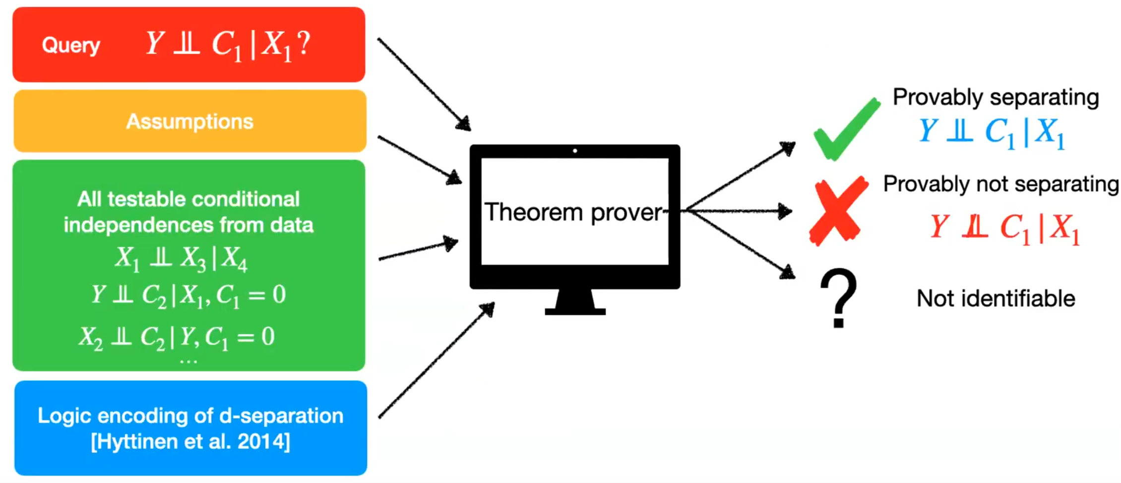
A graphical overview of the object of interest and the quantities that go in the theorem prover is depicted in Figure 1.

Computational side of the method summary

The main focus here is the approach, not implementation, though an implementation is suggested and evaluated. On a high level, computationally the method works as follows:

1. Find all “interesting” subsets of features ordered by risk in ascending order (say using a Random Forest).
2. Consider each subset $A$ from step 1. and do until a satisfying condition is found; otherwise abstain from making a prediction:
   1. Find all conditional independences (or rather independence $p$-values) that involve the target variable (in the source data), and do not (in both source and target data) taking into account Assumptions 1,2 as constraints.
   2. (Magic step) Somehow query the confidence $Y \ind C_1 \mid A$ using the method introduced in (missing reference). [No idea how this works for now].
   3. If the confidence from previous step is high, stop the method and train a regressor of the target variable on source data.

If no subset is found, the method stops and absents from making a prediction. Otherwise, a found subset can provably be used robustly in the target setting just based on the source data.

Final thoughts

The paper defines the domain adaptation problem, lays out the assumptions of the causal generative process in a formal way, and provides a solution to possibly recover sets of separating sets. I still have many questions about the motivation of some of the assumptions and applicability of the model, but this might be due to my inexperience in this field. From the looks of it, the assumptions seem very strict. Additionally, even in this restrictive setting, the algorithm requires to know all conditional independences and potentially considers all possible subsets of the features; though I do not think this is a big issue if we can easily confirm that the assumptions hold. In this case, having a method that works at all, gives guarantees, and does not require to construct a causal graph seems super beneficial.