Notes on (Restricted) Boltzmann Machines

$$ \newcommand{\bzero}{\mathbf{0}} \newcommand{\ba}{\mathbf{a}}\newcommand{\bA}{\mathbf{A}} \newcommand{\bb}{\mathbf{b}}\newcommand{\bB}{\mathbf{B}} \newcommand{\bc}{\mathbf{c}}\newcommand{\bC}{\mathbf{C}} \newcommand{\bd}{\mathbf{d}}\newcommand{\bD}{\mathbf{D}} \newcommand{\be}{\mathbf{e}}\newcommand{\bE}{\mathbf{E}} \newcommand{\bff}{\mathbf{f}}\newcommand{\bF}{\mathbf{F}} \newcommand{\bg}{\mathbf{g}}\newcommand{\bG}{\mathbf{G}} \newcommand{\bh}{\mathbf{h}}\newcommand{\bH}{\mathbf{H}} \newcommand{\bi}{\mathbf{i}}\newcommand{\bI}{\mathbf{I}} \newcommand{\bj}{\mathbf{j}}\newcommand{\bJ}{\mathbf{J}} \newcommand{\bk}{\mathbf{k}}\newcommand{\bK}{\mathbf{K}} \newcommand{\bl}{\mathbf{l}}\newcommand{\bL}{\mathbf{L}} \newcommand{\bm}{\mathbf{m}}\newcommand{\bM}{\mathbf{M}} \newcommand{\bn}{\mathbf{n}}\newcommand{\bN}{\mathbf{N}} \newcommand{\bo}{\mathbf{o}}\newcommand{\bO}{\mathbf{O}} \newcommand{\bp}{\mathbf{p}}\newcommand{\bP}{\mathbf{P}} \newcommand{\bq}{\mathbf{q}}\newcommand{\bQ}{\mathbf{Q}} \newcommand{\br}{\mathbf{r}}\newcommand{\bR}{\mathbf{R}} \newcommand{\bs}{\mathbf{s}}\newcommand{\bS}{\mathbf{S}} \newcommand{\bt}{\mathbf{t}}\newcommand{\bT}{\mathbf{T}} \newcommand{\bu}{\mathbf{u}}\newcommand{\bU}{\mathbf{U}} \newcommand{\bv}{\mathbf{v}}\newcommand{\bV}{\mathbf{V}} \newcommand{\bw}{\mathbf{w}}\newcommand{\bW}{\mathbf{W}} \newcommand{\indep}{\perp \!\!\! \perp} \newcommand{\bx}{\mathbf{x}}\newcommand{\bX}{\mathbf{X}} \newcommand{\by}{\mathbf{y}}\newcommand{\bY}{\mathbf{Y}} \newcommand{\bz}{\mathbf{z}}\newcommand{\bZ}{\mathbf{Z}} \newcommand{\balpha}{\boldsymbol{\alpha}}\newcommand{\bAlpha}{\boldsymbol{\Alpha}} \newcommand{\bbeta}{\boldsymbol{\beta}}\newcommand{\bBeta}{\boldsymbol{\Beta}} \newcommand{\bgamma}{\boldsymbol{\gamma}}\newcommand{\bGamma}{\boldsymbol{\Gamma}} \newcommand{\bdelta}{\boldsymbol{\delta}}\newcommand{\bDelta}{\boldsymbol{\Delta}} \newcommand{\bepsilon}{\boldsymbol{\epsilon}}\newcommand{\bEpsilon}{\boldsymbol{\Epsilon}} \newcommand{\bzeta}{\boldsymbol{\zeta}}\newcommand{\bZeta}{\boldsymbol{\Zeta}} \newcommand{\beeta}{\boldsymbol{\eta}}\newcommand{\bEta}{\boldsymbol{\Eta}} % \beta already taken \newcommand{\btheta}{\boldsymbol{\theta}}\newcommand{\bTheta}{\boldsymbol{\Theta}} \newcommand{\biota}{\boldsymbol{\iota}}\newcommand{\bIota}{\boldsymbol{\Iota}} \newcommand{\bkappa}{\boldsymbol{\kappa}}\newcommand{\bKappa}{\boldsymbol{\Kappa}} \newcommand{\blambda}{\boldsymbol{\lambda}}\newcommand{\bLambda}{\boldsymbol{\Lambda}} \newcommand{\bmu}{\boldsymbol{\mu}}\newcommand{\bMu}{\boldsymbol{\Mu}} \newcommand{\bnu}{\boldsymbol{\nu}}\newcommand{\bNu}{\boldsymbol{\Nu}} \newcommand{\bxi}{\boldsymbol{\xi}}\newcommand{\bXi}{\boldsymbol{\Xi}} \newcommand{\bomikron}{\boldsymbol{\omikron}}\newcommand{\bOmikron}{\boldsymbol{\Omikron}} \newcommand{\bpi}{\boldsymbol{\pi}}\newcommand{\bPi}{\boldsymbol{\Pi}} \newcommand{\brho}{\boldsymbol{\rho}}\newcommand{\bRho}{\boldsymbol{\Rho}} \newcommand{\bsigma}{\boldsymbol{\sigma}}\newcommand{\bSigma}{\boldsymbol{\Sigma}} \newcommand{\btau}{\boldsymbol{\tau}}\newcommand{\bTau}{\boldsymbol{\Tau}} \newcommand{\bypsilon}{\boldsymbol{\ypsilon}}\newcommand{\bYpsilon}{\boldsymbol{\Ypsilon}} \newcommand{\bphi}{\boldsymbol{\phi}}\newcommand{\bPhi}{\boldsymbol{\Phi}} \newcommand{\bchi}{\boldsymbol{\chi}}\newcommand{\bChi}{\boldsymbol{\Chi}} \newcommand{\bpsi}{\boldsymbol{\psi}}\newcommand{\bPsi}{\boldsymbol{\Psi}} \newcommand{\bomega}{\boldsymbol{\omega}}\newcommand{\bOmega}{\boldsymbol{\Omega}} \newcommand{\nA}{\mathbb{A}} \newcommand{\nB}{\mathbb{B}} \newcommand{\nC}{\mathbb{C}} \newcommand{\nD}{\mathbb{D}} \newcommand{\nE}{\mathbb{E}} \newcommand{\nF}{\mathbb{F}} \newcommand{\nG}{\mathbb{G}} \newcommand{\nH}{\mathbb{H}} \newcommand{\nI}{\mathbb{I}} \newcommand{\nJ}{\mathbb{J}} \newcommand{\nK}{\mathbb{K}} \newcommand{\nL}{\mathbb{L}} \newcommand{\nM}{\mathbb{M}} \newcommand{\nN}{\mathbb{N}} \newcommand{\nO}{\mathbb{O}} \newcommand{\nP}{\mathbb{P}} \newcommand{\nQ}{\mathbb{Q}} \newcommand{\nR}{\mathbb{R}} \newcommand{\nS}{\mathbb{S}} \newcommand{\nT}{\mathbb{T}} \newcommand{\nU}{\mathbb{U}} \newcommand{\nV}{\mathbb{V}} \newcommand{\nW}{\mathbb{W}} \newcommand{\nX}{\mathbb{X}} \newcommand{\nY}{\mathbb{Y}} \newcommand{\nZ}{\mathbb{Z}} \newcommand{\cA}{\mathcal{A}} \newcommand{\cB}{\mathcal{B}} \newcommand{\cC}{\mathcal{C}} \newcommand{\cD}{\mathcal{D}} \newcommand{\cE}{\mathcal{E}} \newcommand{\cF}{\mathcal{F}} \newcommand{\cG}{\mathcal{G}} \newcommand{\cH}{\mathcal{H}} \newcommand{\cI}{\mathcal{I}} \newcommand{\cJ}{\mathcal{J}} \newcommand{\cK}{\mathcal{K}} \newcommand{\cL}{\mathcal{L}} \newcommand{\cM}{\mathcal{M}} \newcommand{\cN}{\mathcal{N}} \newcommand{\cO}{\mathcal{O}} \newcommand{\cP}{\mathcal{P}} \newcommand{\cQ}{\mathcal{Q}} \newcommand{\cR}{\mathcal{R}} \newcommand{\cS}{\mathcal{S}} \newcommand{\cT}{\mathcal{T}} \newcommand{\cU}{\mathcal{U}} \newcommand{\cV}{\mathcal{V}} \newcommand{\cW}{\mathcal{W}} \newcommand{\cX}{\mathcal{X}} \newcommand{\cY}{\mathcal{Y}} \newcommand{\cZ}{\mathcal{Z}} \DeclareMathOperator*{\argmax}{argmax~} \DeclareMathOperator*{\argmin}{argmin~} \DeclareMathOperator*{\Tr}{Tr} \DeclareMathOperator*{\Bias}{Bias} \DeclareMathOperator*{\Var}{Var} \newcommand{\Perp}{\perp\!\!\! \perp} \let\dsad\d \renewcommand\d{\, \mathrm{d}} \newcommand{\R}{\mathbb{R}} \newcommand{\N}{\mathbb{N}} \newcommand{\E}{\mathbb{E}} \newcommand{\Eb}[1]{\mathbb{E} \left[ #1 \right]} \newcommand{\F}{\mathcal{F}} \newcommand{\X}{\mathcal{X}} \newcommand{\vocab}[1]{\textbf{\color{blue} #1}} \newcommand{\norm}[1]{\left\lVert#1\right\rVert} \newcommand{\inner}[2]{ \left \langle #1, #2 \right \rangle } \newcommand{\ibra}[1]{\llbracket #1 \rrbracket} \newenvironment{nalign}{ \begin{equation} \begin{aligned} }{ \end{aligned} \end{equation} \ignorespacesafterend } \newcommand{\icol}[1]{ \left(\begin{smallmatrix}#1\end{smallmatrix}\right)% } \newcommand{\cc}[1]{\overline{#1}} \newcommand{\tr}[1]{\text{tr} \left( #1 \right)} \newcommand{\aff}{\text{aff} \,} \newcommand{\ri}{\text{ri} \, } \newcommand{\rb}{\text{rb} \, } \newcommand{\cl}{\text{cl} \, } \newcommand{\conv}{\text{conv} \, } \newcommand{\irow}[1]{ \begin{smallmatrix}(#1)\end{smallmatrix}% } \newcommand\abs[1]{\left \lvert #1 \right \rvert} $$

Outline:

1. Describe the model
2. Prerequisites regarding reading off the conditional independences
   1. Model-specific cond. independences
3. Derive the (log)-likelihood, make a comment why it is so easy.
4. Cover Gibbs sampling in some detail as a reminder
5. Describe Constrastive-Divergence and its Persistent version.
6. Show in code

We deal with a Markov network in an unsupervised setting. It is a generative and undirected model that attempts to model the data distribution $p(\bx)$. This model in its vanilla form only works with binary data. Additionally, it also models the hidden layer as a set of Bernoulli random variables.

The model is characterized by an energy function over the visible variables $\bx$ and hidden variables $\bh$ in the following way:

\[\begin{equation} \begin{split} E(\bx, \bh) = -\bx^\intercal \bw_\bx - \bh^\intercal \bw_\bh - \bx^\intercal W \bh, \end{split} \end{equation}\]

where the weights $\bw_\bx, \bw_\bh$ serve as biases for respective variables, and the weight matrix $W$ is used to relate the observed variables with hidden representations.

Our goal is to learn the weights that minimize the energy over all the training samples, which we can do by, say, using likelihood maximization methods. For that, it is useful to express the energy in a probabilistic fashion. In this case we express it using Boltzmann distribution with a temperature parameter fixed to $T= 1$ in the following way:

\[\begin{equation} \begin{split} p(\bx, \bh) &= \frac{1}{Z(\btheta)} \exp \left ( -E(\bx, \bh) \right ) \\ &= \frac{1}{Z(\btheta)} \exp (\bx^\intercal \bw_\bx + \bh^\intercal \bw_\bh + \bx^\intercal W \bh ) \\ &= \frac{1}{Z(\btheta)} \exp (\bx^\intercal \bw_\bx) \exp(\bh^\intercal \bw_\bh ) \exp(\bx^\intercal W \bh ), \end{split} \end{equation}\]

where we defined the set of all paramters $\btheta := (\bw_\bx, \bw_\bh, W)$ and $Z(\btheta) := \sum_{\bx, \bh} \left ( -E(\bx, \bh) \right )$ is the normalization constant (also known as partition function).

Conditional independences and graphical representation

Due to the structure of the objective, we can pick out conditional independences that will be useful when optimizing the parameters. Now, the way we defined the problem through its objective does not fully inform us about the conditional independnces (unless we manipulate the expression explicitly to separate things out), but the graphical-representation-view does. If we had defined the problem in a graphical way and then defined individual factors, we would be certain that the independence structure would be preserved in the objective function too. Since this is not the path we took, we will recover the graphical view from massaging the objective. For this, rewrite the probability of the system as follows:

\[\begin{equation} \begin{split} p(\bx, \bh) &= \frac{1}{Z(\btheta)} \exp (\bx^\intercal \bw_\bx) \exp(\bh^\intercal \bw_\bh ) \exp(\bx^\intercal W \bh ) \\ &= \frac{1}{Z(\btheta)} \exp (\bx^\intercal \bw_\bx) \exp(\bh^\intercal \bw_\bh ) \exp \left ( \sum_i x_i (W \bh)_i \right ) \\ &= \frac{1}{Z(\btheta)} \exp (\bx^\intercal \bw_\bx) \exp(\bh^\intercal \bw_\bh ) \exp \left ( \sum_i \sum_j w_{ij} x_i h_j \right ) \\ &= \frac{1}{Z(\btheta)} \exp (\bx^\intercal \bw_\bx) \exp(\bh^\intercal \bw_\bh ) \prod_i^D \prod_j^H \exp \left ( w_{ij} x_i h_j \right ) \\ &= \frac{1}{Z(\btheta)}\exp(\bh^\intercal \bw_\bh ) \prod_i^D \underbrace{\left [ \left ( \prod_j^H \exp \left ( w_{ij} h_j \right ) \right )^{x_i} x_i w^{(x)}_i \right]}_{\propto p(x_i \mid \bh)}, \end{split} \end{equation}\]

where in the last equation I joined the unary and binary terms. This last equation precisely shows that given all the hidden units $\bh$, each visibile unit $x_i$ is independent from each other. Analogously, we can show that it holds that $p(h_j \mid \bx)$ is independent among all $j$.

With these conditional independences in mind, we can represent the model in an informative way as a Markov network. To construct the graph, we only need to know the Local Markov Property.

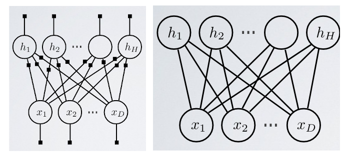
The Local Markov Property holds because we shoed that this holds for the two types of variables that we have: visible $\bx$ and hidden $\bh$. As such, we can draw the graph as depicted in Figure 1. To be more explicit, we also denote the corresponding unary and binary factors.

Deriving the training objective

We will take Maximimum-Likelihood approach to optimize the network weights. It turns out, that because of the conditional independence structure of the model, marginalizing out the hidden variables is particularly easy. To see this, write the likelihood of the data given the parameters $\btheta$ as:

\[\begin{equation} \begin{split} p(\bx) = \sum_{h_1, \dots, h_H} p(\bx, h_1, \dots, h_H), \end{split} \end{equation}\]

where we marginalize over the binary variables $h_i$. Plugging in the joint probability now yields

\[\begin{equation} \begin{split} \sum_{h_1, \dots, h_H} p(\bx, h_1, \dots, h_H) = \sum_{h_1, \dots, h_H} \end{split} \end{equation}\]