Notes on "Categorical Reparameterization with Gumbel-Softmax" (2017)

$$ \newcommand{\bzero}{\mathbf{0}} \newcommand{\ba}{\mathbf{a}}\newcommand{\bA}{\mathbf{A}} \newcommand{\bb}{\mathbf{b}}\newcommand{\bB}{\mathbf{B}} \newcommand{\bc}{\mathbf{c}}\newcommand{\bC}{\mathbf{C}} \newcommand{\bd}{\mathbf{d}}\newcommand{\bD}{\mathbf{D}} \newcommand{\be}{\mathbf{e}}\newcommand{\bE}{\mathbf{E}} \newcommand{\bff}{\mathbf{f}}\newcommand{\bF}{\mathbf{F}} \newcommand{\bg}{\mathbf{g}}\newcommand{\bG}{\mathbf{G}} \newcommand{\bh}{\mathbf{h}}\newcommand{\bH}{\mathbf{H}} \newcommand{\bi}{\mathbf{i}}\newcommand{\bI}{\mathbf{I}} \newcommand{\bj}{\mathbf{j}}\newcommand{\bJ}{\mathbf{J}} \newcommand{\bk}{\mathbf{k}}\newcommand{\bK}{\mathbf{K}} \newcommand{\bl}{\mathbf{l}}\newcommand{\bL}{\mathbf{L}} \newcommand{\bm}{\mathbf{m}}\newcommand{\bM}{\mathbf{M}} \newcommand{\bn}{\mathbf{n}}\newcommand{\bN}{\mathbf{N}} \newcommand{\bo}{\mathbf{o}}\newcommand{\bO}{\mathbf{O}} \newcommand{\bp}{\mathbf{p}}\newcommand{\bP}{\mathbf{P}} \newcommand{\bq}{\mathbf{q}}\newcommand{\bQ}{\mathbf{Q}} \newcommand{\br}{\mathbf{r}}\newcommand{\bR}{\mathbf{R}} \newcommand{\bs}{\mathbf{s}}\newcommand{\bS}{\mathbf{S}} \newcommand{\bt}{\mathbf{t}}\newcommand{\bT}{\mathbf{T}} \newcommand{\bu}{\mathbf{u}}\newcommand{\bU}{\mathbf{U}} \newcommand{\bv}{\mathbf{v}}\newcommand{\bV}{\mathbf{V}} \newcommand{\bw}{\mathbf{w}}\newcommand{\bW}{\mathbf{W}} \newcommand{\bx}{\mathbf{x}}\newcommand{\bX}{\mathbf{X}} \newcommand{\by}{\mathbf{y}}\newcommand{\bY}{\mathbf{Y}} \newcommand{\bz}{\mathbf{z}}\newcommand{\bZ}{\mathbf{Z}} \newcommand{\balpha}{\boldsymbol{\alpha}}\newcommand{\bAlpha}{\boldsymbol{\Alpha}} \newcommand{\bbeta}{\boldsymbol{\beta}}\newcommand{\bBeta}{\boldsymbol{\Beta}} \newcommand{\bgamma}{\boldsymbol{\gamma}}\newcommand{\bGamma}{\boldsymbol{\Gamma}} \newcommand{\bdelta}{\boldsymbol{\delta}}\newcommand{\bDelta}{\boldsymbol{\Delta}} \newcommand{\bepsilon}{\boldsymbol{\epsilon}}\newcommand{\bEpsilon}{\boldsymbol{\Epsilon}} \newcommand{\bzeta}{\boldsymbol{\zeta}}\newcommand{\bZeta}{\boldsymbol{\Zeta}} \newcommand{\beeta}{\boldsymbol{\eta}}\newcommand{\bEta}{\boldsymbol{\Eta}} % \beta already taken \newcommand{\btheta}{\boldsymbol{\theta}}\newcommand{\bTheta}{\boldsymbol{\Theta}} \newcommand{\biota}{\boldsymbol{\iota}}\newcommand{\bIota}{\boldsymbol{\Iota}} \newcommand{\bkappa}{\boldsymbol{\kappa}}\newcommand{\bKappa}{\boldsymbol{\Kappa}} \newcommand{\blambda}{\boldsymbol{\lambda}}\newcommand{\bLambda}{\boldsymbol{\Lambda}} \newcommand{\bmu}{\boldsymbol{\mu}}\newcommand{\bMu}{\boldsymbol{\Mu}} \newcommand{\bnu}{\boldsymbol{\nu}}\newcommand{\bNu}{\boldsymbol{\Nu}} \newcommand{\bxi}{\boldsymbol{\xi}}\newcommand{\bXi}{\boldsymbol{\Xi}} \newcommand{\bomikron}{\boldsymbol{\omikron}}\newcommand{\bOmikron}{\boldsymbol{\Omikron}} \newcommand{\bpi}{\boldsymbol{\pi}}\newcommand{\bPi}{\boldsymbol{\Pi}} \newcommand{\brho}{\boldsymbol{\rho}}\newcommand{\bRho}{\boldsymbol{\Rho}} \newcommand{\bsigma}{\boldsymbol{\sigma}}\newcommand{\bSigma}{\boldsymbol{\Sigma}} \newcommand{\btau}{\boldsymbol{\tau}}\newcommand{\bTau}{\boldsymbol{\Tau}} \newcommand{\bypsilon}{\boldsymbol{\ypsilon}}\newcommand{\bYpsilon}{\boldsymbol{\Ypsilon}} \newcommand{\bphi}{\boldsymbol{\phi}}\newcommand{\bPhi}{\boldsymbol{\Phi}} \newcommand{\bchi}{\boldsymbol{\chi}}\newcommand{\bChi}{\boldsymbol{\Chi}} \newcommand{\bpsi}{\boldsymbol{\psi}}\newcommand{\bPsi}{\boldsymbol{\Psi}} \newcommand{\bomega}{\boldsymbol{\omega}}\newcommand{\bOmega}{\boldsymbol{\Omega}} \newcommand{\nA}{\mathbb{A}} \newcommand{\nB}{\mathbb{B}} \newcommand{\nC}{\mathbb{C}} \newcommand{\nD}{\mathbb{D}} \newcommand{\nE}{\mathbb{E}} \newcommand{\nF}{\mathbb{F}} \newcommand{\nG}{\mathbb{G}} \newcommand{\nH}{\mathbb{H}} \newcommand{\nI}{\mathbb{I}} \newcommand{\nJ}{\mathbb{J}} \newcommand{\nK}{\mathbb{K}} \newcommand{\nL}{\mathbb{L}} \newcommand{\nM}{\mathbb{M}} \newcommand{\nN}{\mathbb{N}} \newcommand{\nO}{\mathbb{O}} \newcommand{\nP}{\mathbb{P}} \newcommand{\nQ}{\mathbb{Q}} \newcommand{\nR}{\mathbb{R}} \newcommand{\nS}{\mathbb{S}} \newcommand{\nT}{\mathbb{T}} \newcommand{\nU}{\mathbb{U}} \newcommand{\nV}{\mathbb{V}} \newcommand{\nW}{\mathbb{W}} \newcommand{\nX}{\mathbb{X}} \newcommand{\nY}{\mathbb{Y}} \newcommand{\nZ}{\mathbb{Z}} \newcommand{\cA}{\mathcal{A}} \newcommand{\cB}{\mathcal{B}} \newcommand{\cC}{\mathcal{C}} \newcommand{\cD}{\mathcal{D}} \newcommand{\cE}{\mathcal{E}} \newcommand{\cF}{\mathcal{F}} \newcommand{\cG}{\mathcal{G}} \newcommand{\cH}{\mathcal{H}} \newcommand{\cI}{\mathcal{I}} \newcommand{\cJ}{\mathcal{J}} \newcommand{\cK}{\mathcal{K}} \newcommand{\cL}{\mathcal{L}} \newcommand{\cM}{\mathcal{M}} \newcommand{\cN}{\mathcal{N}} \newcommand{\cO}{\mathcal{O}} \newcommand{\cP}{\mathcal{P}} \newcommand{\cQ}{\mathcal{Q}} \newcommand{\cR}{\mathcal{R}} \newcommand{\cS}{\mathcal{S}} \newcommand{\cT}{\mathcal{T}} \newcommand{\cU}{\mathcal{U}} \newcommand{\cV}{\mathcal{V}} \newcommand{\cW}{\mathcal{W}} \newcommand{\cX}{\mathcal{X}} \newcommand{\cY}{\mathcal{Y}} \newcommand{\cZ}{\mathcal{Z}} \DeclareMathOperator*{\argmax}{argmax~} \DeclareMathOperator*{\argmin}{argmin~} \DeclareMathOperator*{\Tr}{Tr} \DeclareMathOperator*{\Bias}{Bias} \DeclareMathOperator*{\Var}{Var} \newcommand{\Perp}{\perp\!\!\! \perp} \let\dsad\d \renewcommand\d{\mathrm{d}} \newcommand{\R}{\mathbb{R}} \newcommand{\N}{\mathbb{N}} \newcommand{\E}{\mathbb{E}} \newcommand{\Eb}[1]{\mathbb{E} \left[ #1 \right]} \newcommand{\F}{\mathcal{F}} \newcommand{\X}{\mathcal{X}} \newcommand{\vocab}[1]{\textbf{\color{blue} #1}} \newcommand{\norm}[1]{\left\lVert#1\right\rVert} \newcommand{\inner}[2]{ \left \langle #1, #2 \right \rangle } \newcommand{\ibra}[1]{\llbracket #1 \rrbracket} \newenvironment{nalign}{ \begin{equation} \begin{aligned} }{ \end{aligned} \end{equation} \ignorespacesafterend } \newcommand{\icol}[1]{ \left(\begin{smallmatrix}#1\end{smallmatrix}\right)% } \newcommand{\cc}[1]{\overline{#1}} \newcommand{\tr}[1]{\text{tr} \left( #1 \right)} \newcommand{\aff}{\text{aff} \,} \newcommand{\ri}{\text{ri} \, } \newcommand{\rb}{\text{rb} \, } \newcommand{\cl}{\text{cl} \, } \newcommand{\conv}{\text{conv} \, } \newcommand{\irow}[1]{ \begin{smallmatrix}(#1)\end{smallmatrix}% } \newcommand\abs[1]{\lvert #1 \rvert} $$

In this post I continue looking into stochastic neural network training, and look into the famous two papers that concurrently came up with similar conceptual results (missing reference), (missing reference). Here the objective is very simple: allow for differentiating of sampling operation in backpropagation.

Motivation

The motivation is that reparameterization trick showed the world that having learnable-parameter-dependent noise in the computation graph is fine as long as the distribution from which the noise is sampled is reparameterizable, deterministic and differentiable.

But many applications require introducing discrete nodes into the computation graph. One example would be networks that involve expectations over discrete variables (think SSL-VAE).

This inability to backprop through discrete is problematic because we need to resort to score-like estimators that have extremely high variance. However, one approach that is taken in practice is to relax discrete functions into their continuous counterparts. This is the approach that is taken in the paper.

Gumbel-Max trick

Apparently well-known way to sample from discrete distribution is to use the Gumbel-max trick. How else can we sample from a categorical? Well using the simplest way of inverse transform sampling, where we can simply construct the CDF of the discrete value, and push uniform samples through inverse CDF function. However, Gumbel-Max trick uses argmax function, which can be relaxed and is (probably?) the reason why this sampling approach is used.

I will simply introduce the trick and show that it enjoys useful properties.

Definition (Gumbel random variable) A continuous Gumbel random variable $G$ with support on the whole real line has PDF $\cG(x; \mu, \beta) = \frac{1}{\beta} e^{-z -e^{-z}}$ with $z = \frac{x - \mu}{\beta}$.

But we mostly use the standard gumbel, i.e. $\cG(0,1)$.

Notation (Standard Gumbel r.v.) We denote $G$ to be the PDF of 0-location and 1-scale Gumbel r.v., i.e. $\cG(x) := g(x; 0, 1) = e^{-x - e^{-x}}$.

Assuming we can sample from standard Gumbel, we can then finally sample from a categorical distribution by using samples from a Gumbel distribution, which gives rise to the Gumbel-max trick. Concretely, a discrete random variable following a categorical distribution over $n$ states $X \sim \text{cat}(\alpha_1, \dots, \alpha_n)$ can be sampled from by drawing $n$ samples $\bg = (g_1, \dots, g_n)$ from a standard Gumbel distribution, adding the samples element-wise to the log-probabilities $\balpha$ and taking the argmax.

Before seeing why it works, we will need to use integration by substitution and CDF of a Gumbel distribution.

Proof. Substitute $u = e^{-x}$ and integrate.

To show that this holds, we show a related statement (where wlog we consider only the probability that the argmax will be the first element, but of course this holds for other indices too).

Proof.

Then the proof for the validity of Gumbel-Max trick (Proposition 1) follows immediately if we take $\alpha_i := \log \alpha_i$, in which case

as desired!

Sampling from Gumbel distribution: Inverse Transform Sampling

Now that we know how to sample from a categorical distribution using samples from Gumbel distribution, we first need to generate samples from a Gumbel distribution. To do that, we use the intuitive way of sampling using inverse transform sampling. It sounds a bit mindless to go from the simplest way of inverse transform sampling to using Gumbel samples, only to return to the need to use inverse sampling, but this time to acquire samples not from a discrete, but from a Gumbel distribution. But it will all be worth it once we relax the argmax operator and have backpropable loss.

In order to carry out inverse transform sampling procedure, we need to compute inverse CDF of the Gumbel distribution. This will guarantee that the PDF of this newly-computed random variable will correspond to Gumbel density. Since we know the CDF of Gumbel has an easy analytic form (and as it happens the inverse), sampling from Gumbel is then as easy as sampling from uniform distribution.

Relaxing the $\text{argmax}$

Now that we know how to sample from discrete using Gumbel-Max trick, we can actually make use of $\text{softmax}$, which is a continuous soft argmax, contrary to what its name indicates. In its base form it is defined as

and it follows that as some element of $\balpha$ goes to infinity, the $\text{softmax} \to \text{argmax}$. However, we can actually ensure that $\text{softmax}$ approaches $\text{argmax}$ in an easier way, by simply scaling each element of $\balpha$ by some $\frac{1}{\lambda}$. Then the following holds

Proof source. Wlog assume $x_1 = \max_i x_i$, then \(\begin{equation} \begin{split} L = \lim_{\lambda \to 0} \text{softmax}(\balpha / \lambda)_i = \lim_{\lambda \to 0} \text{softmax} \left( \frac{ \balpha}{\lambda} \right)_i = \begin{cases} \lim_{\lambda \to 0} \left( \frac{\exp{\alpha_1 / \lambda} }{\sum \exp {\alpha_j / \lambda}} = \frac{\exp{(\alpha_1 - \alpha_1) / \lambda} }{\sum \exp {(\alpha_j - \alpha_i)/ \lambda}} \right) = 1& \text{if } i = 1 \\ \lim_{\lambda \to 0} \left( \frac{\exp{\alpha_i / \lambda} }{\sum \exp {\alpha_j / \lambda}} = \frac{\exp{(\alpha_i - \alpha_1) / \lambda} }{\sum \exp {(\alpha_j - \alpha_i)/ \lambda}} \right) = 0 & \text{if } i \neq 1 \end{cases}, \end{split} \end{equation}\)

Thus, introducing this parameter $\lambda$ determines how much the $\text{softmax}$ approximates $\text{argmax}$ ( $\lambda = 0$ corresponding to discrete case, and $\lambda \to \infty$ corresponding to uniform case).

This gives rise to the $\text{Concrete}$ (or $\text{Gumbel-Softmax}$) distribution.

So now we have all the ingredients to make the $\text{argmax}$ backpropable: in the limit $\lambda \to 0$, we recover the discrete $\text{argmax}$, and if we simply sample from $\text{argmax}$, we directly sample from categorical. Thus, we use samples from $\text{Concrete}$ as a continuos surrogate to Gumbel-Max procedure.

Backpropagationability(!)

To show the benefit in backproping through sampling of a discrete distribution. Consider the following optimization objective over $n$ parameters $\balpha \in \R^n_+$:

In such a case, using the samples attained from inverse transform sampling (which requires to evaluate a discrete inverse CDF function), as well as using Gumbel-Max trick with hard $\text{argmax}$ leads to 0 gradient everywhere except at the boundary points where it is undefined:

But using the $\text{Concrete}$ as a relaxation with temperature parameter $\lambda$ yields:

which now poses no problem due to continuous $\text{softmax}$.

Implementing $\text{Concrete}$

To implement the $\text{Concrete}$, all we need is to sample from Gumbel, which we know how to do based on inverse sampling and apply $\lambda$-scaled $\text{softmax}$. To sample from standard gumbel:

def sample_from_gumbel(n_samples, n_dims):
    # add epsilon to avoid 0-probs
    uniforms = np.clip(np.random.random(size=(n_samples, n_dims)), 1e-2, 1) 
    return -np.log(-np.log(uniforms))

and to then sample from categorical:

def sample_from_categorical_using_concrete(n_samples, probs, temp_lambda = 1.0):
    n_categories = probs.shape[0]
    
    gumbels = sample_from_gumbel(n_samples, n_categories)

    # Note that softmax( {x}_i=1^n - c)_j = softmax( {x}_i)_j for a constant c,
    # i.e. subtracting the max from the softmax yields the same result but is 
    # more numerically stable
    concrete_args = (np.log(probs) + gumbels) / temp_lambda
    max_arg_vals = np.max(concrete_args, axis=1, keepdims=True)

    exp_logits = np.exp(concrete_args - max_arg_vals)
    soft_argmax_samples = exp_logits / (np.sum(exp_logits,axis=1,keepdims=True))

    return soft_argmax_samples

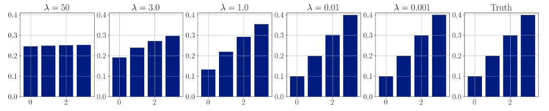
We can then confirm that the logic of warying $\lambda$ matches the derived results empirically (we assume $X \sim \text{cat}(0.1, 0.2, 0.3, 0.4)$) by sampling from the $\text{Concrete}$ and then taking the mean of the soft-samples:

A difference between the papers when considering VAEs

One interesting difference between the two papers is their approach of applying VAEs on log-evidence lower bound when the approximate posterior $q(\bz \mid \bx)$ is over a discrete variable $\bz$. Suppose we follow the standard procedure of variational inference by writing out the ELBO:

If we had a way to optimize it through gradient descent, we would be done. Since this is not the case and we rely on $\text{argmax}$ relaxations there are two ways how to optimize the above expression:

1. Relax the approximate poterior $Q(\bz \mid \bx) \overset{\text{relax}}{\rightsquigarrow} \text{concrete}(f(\bx), \lambda)$, but assume that categorical discrete prior $P(\bz)$ remains categorical. This is the approach taken by [1]. In this case the above expression is not an ELBO anymore, because evaluating KL divergence between distinct families of distributions does not guarantee to lower bound the evidence anymore. However, the authors note that this approach still works.
2. Relax the approximate posterior in the same was as before, but now also relax the prior to be a $\text{concrete}$ with possibly different temperature value. This then leads to a valid lower bound and is the approach taken in [2].

The safe choice is (2), but the one easier to implement and, I guess, having less “variance” (this is not a fair comparison anyway, hence the quatation marks), due to closed form solution of the KL term, is the (1).

Toy task: Variational-Bayes Auto Encoder using discrete latent variables

To see if our implementation makes sense, I will try to apply sampling from $\text{Concrete}$ on toy task which allows to compute the expectation exactly by having only 10 variables. For this I simply take MNIST data and train a variational autoencoder with a 10-dimensional one-hot bottleneck $\bz$ represented by a categorical random variable. This is a special case of the experiment done in [2], but in their case exact marginalization was infeasible to compute. Formally, assuming no relaxations for now, the generative and inference models can be described as follows (assuming a single datapoint):

Version #1: Relax only the sampling $\Rightarrow$ not a variational bound

In the simplest case, we simply replace the approximate posterior $Q(\bz \mid \bx)$ with a concrete distribution parameterized by a NN, $Q(\bz \mid \bx) \overset{\text{relax}}{\rightsquigarrow} \text{concrete}(\balpha_q(\bx), \lambda_x)$, where a NN $\balpha_q(\cdot)$ outputs the parameters given $\bx$. In this case the no-longer-bound reads: