Notes on "Causal Influence Detection for Improving Efficiency in Reinforcement Learning" (2021)

$$ \newcommand{\bzero}{\mathbf{0}} \newcommand{\ba}{\mathbf{a}}\newcommand{\bA}{\mathbf{A}} \newcommand{\bb}{\mathbf{b}}\newcommand{\bB}{\mathbf{B}} \newcommand{\bc}{\mathbf{c}}\newcommand{\bC}{\mathbf{C}} \newcommand{\bd}{\mathbf{d}}\newcommand{\bD}{\mathbf{D}} \newcommand{\be}{\mathbf{e}}\newcommand{\bE}{\mathbf{E}} \newcommand{\bff}{\mathbf{f}}\newcommand{\bF}{\mathbf{F}} \newcommand{\bg}{\mathbf{g}}\newcommand{\bG}{\mathbf{G}} \newcommand{\bh}{\mathbf{h}}\newcommand{\bH}{\mathbf{H}} \newcommand{\bi}{\mathbf{i}}\newcommand{\bI}{\mathbf{I}} \newcommand{\bj}{\mathbf{j}}\newcommand{\bJ}{\mathbf{J}} \newcommand{\bk}{\mathbf{k}}\newcommand{\bK}{\mathbf{K}} \newcommand{\bl}{\mathbf{l}}\newcommand{\bL}{\mathbf{L}} \newcommand{\bm}{\mathbf{m}}\newcommand{\bM}{\mathbf{M}} \newcommand{\bn}{\mathbf{n}}\newcommand{\bN}{\mathbf{N}} \newcommand{\bo}{\mathbf{o}}\newcommand{\bO}{\mathbf{O}} \newcommand{\bp}{\mathbf{p}}\newcommand{\bP}{\mathbf{P}} \newcommand{\bq}{\mathbf{q}}\newcommand{\bQ}{\mathbf{Q}} \newcommand{\br}{\mathbf{r}}\newcommand{\bR}{\mathbf{R}} \newcommand{\bs}{\mathbf{s}}\newcommand{\bS}{\mathbf{S}} \newcommand{\bt}{\mathbf{t}}\newcommand{\bT}{\mathbf{T}} \newcommand{\bu}{\mathbf{u}}\newcommand{\bU}{\mathbf{U}} \newcommand{\bv}{\mathbf{v}}\newcommand{\bV}{\mathbf{V}} \newcommand{\bw}{\mathbf{w}}\newcommand{\bW}{\mathbf{W}} \newcommand{\bx}{\mathbf{x}}\newcommand{\bX}{\mathbf{X}} \newcommand{\by}{\mathbf{y}}\newcommand{\bY}{\mathbf{Y}} \newcommand{\bz}{\mathbf{z}}\newcommand{\bZ}{\mathbf{Z}} \newcommand{\balpha}{\boldsymbol{\alpha}}\newcommand{\bAlpha}{\boldsymbol{\Alpha}} \newcommand{\bbeta}{\boldsymbol{\beta}}\newcommand{\bBeta}{\boldsymbol{\Beta}} \newcommand{\bgamma}{\boldsymbol{\gamma}}\newcommand{\bGamma}{\boldsymbol{\Gamma}} \newcommand{\bdelta}{\boldsymbol{\delta}}\newcommand{\bDelta}{\boldsymbol{\Delta}} \newcommand{\bepsilon}{\boldsymbol{\epsilon}}\newcommand{\bEpsilon}{\boldsymbol{\Epsilon}} \newcommand{\bzeta}{\boldsymbol{\zeta}}\newcommand{\bZeta}{\boldsymbol{\Zeta}} \newcommand{\beeta}{\boldsymbol{\eta}}\newcommand{\bEta}{\boldsymbol{\Eta}} % \beta already taken \newcommand{\btheta}{\boldsymbol{\theta}}\newcommand{\bTheta}{\boldsymbol{\Theta}} \newcommand{\biota}{\boldsymbol{\iota}}\newcommand{\bIota}{\boldsymbol{\Iota}} \newcommand{\bkappa}{\boldsymbol{\kappa}}\newcommand{\bKappa}{\boldsymbol{\Kappa}} \newcommand{\blambda}{\boldsymbol{\lambda}}\newcommand{\bLambda}{\boldsymbol{\Lambda}} \newcommand{\bmu}{\boldsymbol{\mu}}\newcommand{\bMu}{\boldsymbol{\Mu}} \newcommand{\bnu}{\boldsymbol{\nu}}\newcommand{\bNu}{\boldsymbol{\Nu}} \newcommand{\bxi}{\boldsymbol{\xi}}\newcommand{\bXi}{\boldsymbol{\Xi}} \newcommand{\bomikron}{\boldsymbol{\omikron}}\newcommand{\bOmikron}{\boldsymbol{\Omikron}} \newcommand{\bpi}{\boldsymbol{\pi}}\newcommand{\bPi}{\boldsymbol{\Pi}} \newcommand{\brho}{\boldsymbol{\rho}}\newcommand{\bRho}{\boldsymbol{\Rho}} \newcommand{\bsigma}{\boldsymbol{\sigma}}\newcommand{\bSigma}{\boldsymbol{\Sigma}} \newcommand{\btau}{\boldsymbol{\tau}}\newcommand{\bTau}{\boldsymbol{\Tau}} \newcommand{\bypsilon}{\boldsymbol{\ypsilon}}\newcommand{\bYpsilon}{\boldsymbol{\Ypsilon}} \newcommand{\bphi}{\boldsymbol{\phi}}\newcommand{\bPhi}{\boldsymbol{\Phi}} \newcommand{\bchi}{\boldsymbol{\chi}}\newcommand{\bChi}{\boldsymbol{\Chi}} \newcommand{\bpsi}{\boldsymbol{\psi}}\newcommand{\bPsi}{\boldsymbol{\Psi}} \newcommand{\bomega}{\boldsymbol{\omega}}\newcommand{\bOmega}{\boldsymbol{\Omega}} \newcommand{\nA}{\mathbb{A}} \newcommand{\nB}{\mathbb{B}} \newcommand{\nC}{\mathbb{C}} \newcommand{\nD}{\mathbb{D}} \newcommand{\nE}{\mathbb{E}} \newcommand{\nF}{\mathbb{F}} \newcommand{\nG}{\mathbb{G}} \newcommand{\nH}{\mathbb{H}} \newcommand{\nI}{\mathbb{I}} \newcommand{\nJ}{\mathbb{J}} \newcommand{\nK}{\mathbb{K}} \newcommand{\nL}{\mathbb{L}} \newcommand{\nM}{\mathbb{M}} \newcommand{\nN}{\mathbb{N}} \newcommand{\nO}{\mathbb{O}} \newcommand{\nP}{\mathbb{P}} \newcommand{\nQ}{\mathbb{Q}} \newcommand{\nR}{\mathbb{R}} \newcommand{\nS}{\mathbb{S}} \newcommand{\nT}{\mathbb{T}} \newcommand{\nU}{\mathbb{U}} \newcommand{\nV}{\mathbb{V}} \newcommand{\nW}{\mathbb{W}} \newcommand{\nX}{\mathbb{X}} \newcommand{\nY}{\mathbb{Y}} \newcommand{\nZ}{\mathbb{Z}} \newcommand{\cA}{\mathcal{A}} \newcommand{\cB}{\mathcal{B}} \newcommand{\cC}{\mathcal{C}} \newcommand{\cD}{\mathcal{D}} \newcommand{\cE}{\mathcal{E}} \newcommand{\cF}{\mathcal{F}} \newcommand{\cG}{\mathcal{G}} \newcommand{\cH}{\mathcal{H}} \newcommand{\cI}{\mathcal{I}} \newcommand{\cJ}{\mathcal{J}} \newcommand{\cK}{\mathcal{K}} \newcommand{\cL}{\mathcal{L}} \newcommand{\cM}{\mathcal{M}} \newcommand{\cN}{\mathcal{N}} \newcommand{\cO}{\mathcal{O}} \newcommand{\cP}{\mathcal{P}} \newcommand{\cQ}{\mathcal{Q}} \newcommand{\cR}{\mathcal{R}} \newcommand{\cS}{\mathcal{S}} \newcommand{\cT}{\mathcal{T}} \newcommand{\cU}{\mathcal{U}} \newcommand{\cV}{\mathcal{V}} \newcommand{\cW}{\mathcal{W}} \newcommand{\cX}{\mathcal{X}} \newcommand{\cY}{\mathcal{Y}} \newcommand{\cZ}{\mathcal{Z}} \DeclareMathOperator*{\argmax}{argmax~} \DeclareMathOperator*{\argmin}{argmin~} \DeclareMathOperator*{\Tr}{Tr} \DeclareMathOperator*{\Bias}{Bias} \DeclareMathOperator*{\Var}{Var} \newcommand{\Perp}{\perp\!\!\! \perp} \let\dsad\d \renewcommand\d{\mathrm{d}} \newcommand{\R}{\mathbb{R}} \newcommand{\N}{\mathbb{N}} \newcommand{\E}{\mathbb{E}} \newcommand{\Eb}[1]{\mathbb{E} \left[ #1 \right]} \newcommand{\F}{\mathcal{F}} \newcommand{\X}{\mathcal{X}} \newcommand{\vocab}[1]{\textbf{\color{blue} #1}} \newcommand{\norm}[1]{\left\lVert#1\right\rVert} \newcommand{\inner}[2]{ \left \langle #1, #2 \right \rangle } \newcommand{\ibra}[1]{\llbracket #1 \rrbracket} \newenvironment{nalign}{ \begin{equation} \begin{aligned} }{ \end{aligned} \end{equation} \ignorespacesafterend } \newcommand{\icol}[1]{ \left(\begin{smallmatrix}#1\end{smallmatrix}\right)% } \newcommand{\cc}[1]{\overline{#1}} \newcommand{\tr}[1]{\text{tr} \left( #1 \right)} \newcommand{\aff}{\text{aff} \,} \newcommand{\ri}{\text{ri} \, } \newcommand{\rb}{\text{rb} \, } \newcommand{\cl}{\text{cl} \, } \newcommand{\conv}{\text{conv} \, } \newcommand{\irow}[1]{ \begin{smallmatrix}(#1)\end{smallmatrix}% } \newcommand\abs[1]{\lvert #1 \rvert} $$

In this post I summarize “Causal Influence Detection for Improving Efficiency in Reinforcement Learning” (missing reference) – a method that allows to infer whether an RL agent’s actions have a causal influence on entities in the environment. This is particularly useful if the the observations of the environment are already factorized into entities, and the task of the problem is related to these entities. This is the case in the robotic tasks considered in the paper, where the ability to manipulate the entities directly translates into the ability to solve various tasks.

In this paper, a score for an action’s influence on an entity is proposed (locally, conditioned on a state of the environment). If we accept a certain measure of having control over an entity, measuring influence boils down to testing statistical conditional dependence between action and an entity of interest given the state. Conditional mutual information is used to quantify this dependence, though a few approximations are made to make this feasible.

As a result, the method reliably indicates control of action over an entity, achieves improved sampling efficiency, and serves as a good exploration

Motivation

Most RL methods have the advantage of generality, which makes them fit for a wide range of tasks. The disadvantage of this is that it makes them sample-inefficient precisely because it is not known beforehand what data are useful for learning. If we assume some structure about the world, we can make learning faster. If we operate in, say, the physical world, it can be viewed as a composition of independent blocks that interact infrequently. In this case,

The main goal is to formalize the notion of influence, and find a way to quantify it. If we know all the entities, we can either impose the agent to prefer states where the influence is present, or make it an option for the agent to exploit this information.

Assumptions of environments

These are the main assumptions about the environment:

• The environement is representable as a Markov decision process, represented as a tuple $(\cS, \cA, 3P, \cR, \gamma)$ seems like having $\gamma$ here is not standard?, with ordered arguments as: state space, action space, transition probabiltiy distribution, reward function and the discount factor.
• The state space is factorized in entities, i.e. the state space $\cS = \cS_1 \times \dots \times \cS_n$, where each $\cS_i$ represents an entities state; this could be state of a robotic arm, for instance. This assumption makes the job of causal detection easier, since we do not need to extract the entities from the state.

In essence, the main problem that the paper addresses, is the causal interaction discovery between entities locally (that is, in a specific timestep), rather than globally, where all states could influence all others, in theory.

Background

There are a few things we need to define clearly (given here on a high level):

1. How cause and effect are quantified
2. How the interactions are represented

Causal Graphical Models

We represent the causal influence of states on other states by a causal graphical model. In particular, if we look at the global model, then we can look at the transition between $S_t$ and $S_{t+1}$ mediated by the action $A_t$. This gives a causal structure, where a state at the next timestamp, $A_{t+1}$ is caused by the action $A_t$. Additionally, since all the further states could be caused by some other state (not necessarily in one timestep), we can pair up all the states with a directed edge; of course such a pairing might be wrong if there are some lonely states that could potentially not visit other states even in theory.

Concretely, we can construct a graph of transitions $\cG := (\cV, \cE)$, where the nodes are taken as $\cV = { S_1, \dots, S_n, A, S_1’, \dots, S_n’ }$ where $S_i’$ indicates $i$-th proceeding state, and there is a directed edge from a node $X$ to a node $Y$ iff $X$ causes $Y$. Then, we assume, that the probability distribution over the nodes $P_\cV$ is Markovian (it factorizes into independent factors dictated by the graphical model). We don’t assume faithfulness?.

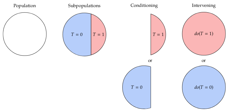
One of the differences between a probabilistic graphical model (PGM) and a CGM, is that one can model interventions. As an example, in PGM we can compute conditional distributions by making use of the joint over all the variables. But there is no rule for computing $\text{do}$ operation, where we can set a r.v. to a state. This not clear; it’s not clear what the setting of a variable means in terms of its influence of other variables

Then, their argument is that the causal graph is not fully connected locally (per timestep). If we knew what states can be influenced, we would not need to concern ourselves of considering these interactions. This is the main goal of this work: to recover the local causal model, a CGM that conditions on a set of vertices of the graph.

Formally, the Local Causal Graphical Model (LCGM) is defined as follows

Intuitively, there is an edge from action A to an entity $S’_j$ in the following step, if there is an action that when “computing” that entity’s state depends on that action. For instance, in a case of a task involving a robotic arm and an object with a goal of transporting an item, if the object is far away then there is no edge from the action to object entity precisely because there is zero action-dependent computation. In contrast, when we are nearby, there can be some actions that actually change the position of the object. In that case, the edge is present.

Why don’t we also delete notes that are useless from the graph? I mean, the nodes can remain, they just won’t influence anything else..

Elaborate on this definition

See Figure 2 for a comparison between a CGM and a LCGM.

The cause of an effect

They distinguish between two ways to address the actual causation problem: the “normative world test” and “but-for test”.

Normative world test

One could try to answer such a question by reasoning what would have happened to $B$ were the action $A = a$ not performed. They write that humans would contrast the actual outcome with a normal outcome, But I guess all that matters here is whether in that case $B \neq b$ in that case. There are multiple challanges of answering such a question:

1. It requires imagining an alternative world with counterfactuals; a world where $A = a$ did not happen.
2. It requires to imagine a world where the agent was not a participant. This is weird. Couldn’t we just image an alternative action and see if that leads to the same conclusion that $B =b$?

But-for test

Another way to answering the queston could be to ask if the effect $B = b$ could have only been caused by an action $A =a$. This of course is not always the case, e.g. when there are multiple ways to cause the effect $B = b$.

Causal influence detection

We finally get to the meat of the paper: causal influence detection.

Simply put, we say that an agent in some state $s$ is in control of state $s’$, if the state $s’$ could be reached using an action from the state $s$. The requirement of all possible interventions is the result of the “but-for” test requirement: if an agent can influence can influence one state, then even if it does not end up in the state, we still consider agent’s influence over the former state. The requirement of policy’s full support is simply to ensure that influence is possible however unlikely.

Next, it is claimed that if there is one policy that is in control of a state (over all possible interventions), then this holds for all other policies of full support (over all possible interventions). Intuitively this is clear when we consider the “but-for” actual causation test.

Measuring causal action influence (Measuring control)

With the notion of control in place, we can formalize a quantity that measures causal influence that an action has a at state $S = s$ on the $j$-th entity. Based on Definition 1, we said that that an agent is in control if there is a statistical association between an action and an entity given the current state. In this work, they measure the dependence by conditional mutual information that is zero only in the case where there is no dependence. This can be written as a function of current state $s$ and the entity index $j$ (in the paper they write the entity index as a superscript; I just made it more explicit) as

\[\begin{equation} \begin{split} \text{CAI}(\bs, j) := \text{mutual-information}(A; S'_j \mid \bs) &= \text{D}_{\text{KL}} \left ( P(A, S'_j \mid \bs) \mid \mid P(A) \, \otimes \, P(S_j' \mid \bs) \right) \\ &= \E_{\ba, \bs_j' \sim P_{A, S_j'}} \left [ \log \frac{P(\ba, \bs'_j \mid \bs)}{P(\bs_j' \mid \bs)} \right] \\ &= \E_{\ba \sim \pi} \left [ \text{D}_{\text{KL}}\left (P({S_j' \mid \bs, \ba}) \mid \mid P(S_j' \mid \bs) \right) \right], \end{split} \end{equation}\]

where the last equation is showed in the paper. If $\text{CAI}$ is zero, it means that for (almost) all actions the transition distribution over the $j$-th entity’s state when taking action into account is identical to the transition distribution when the action is not specified.

Relating CAI score to other measures (in progress)

A few related works include (not really sure how most of these work):

1. Transfer entropy. No idea what this is
   1. Local transfer entropy.
2. Causal strength. Has some advantage over other measures. It was shown that CAI is a pointwise version of this measure for policies that don’t condtion on $S$. Hmm.
3. Empowerment. This basically biases the model to prefer states of maximal influence over the environment. Not entirely sure how this relates to causality.
4. Controllability. We can write the $\text{CAI}$ score as $\nH[S_j’ \mid \bs] - \nH[S’_j \mid A, \bs]$, i.e. as a difference between the intrinsic system’s entropy and the entropy that is still there after an action is known. If the action reduces the uncertainty by a lot, then the score is higher, and is upper-bounded by the system’s intrinsic entropy. (This is cool intuition!).

Approximating CAI (quantifying control approximately)